What Is CFDEM®coupling?
CFDEM®coupling is an advanced simulation software developed by DCS Computing, which combines Discrete Element Method (DEM) and Computational Fluid Dynamics (CFD) technologies to model particle-fluid interactions with precision.
How does CFDEM®coupling work?
Since the release 7.1.0 fully coupled simulations can run on GPU as well, giving the same physics a significant speed-up for large cases without changing your setup.
Already on CFDEM®coupling-PUBLIC or LIGGGHTS®? Aspherix® & CFDEM®coupling is the next stage of that same lineage. It is built by the original team on new architecture, with a GUI in place of script-driven setup, GPU support, and two major releases a year. Read our blog article "From LIGGGHTS to Aspherix" for more information on that topic.
Once the fluid carries a real share of the momentum, heat, or mass in your process, both phases need to be solved together. CFDEM®coupling pairs Aspherix®'s DEM solver with a CFD solver and exchanges data between them at every coupling step, covering both unresolved (particle-averaged, for large particle counts) and resolved (particle-scale flow) regimes.
Beyond momentum coupling, it models the physics that real processes add on top: multiphase flows, heat transfer, evaporation and liquid film/transport, spray formation, and chemical reactions, combined as needed for your case.
This flexibility is why CFDEM®coupling shows up across such different processes: pharmaceutical granulation and drying, blast furnace burden and thermal transfer, battery drying, sediment transport, and, as with The Ocean Cleanup, tracking waterborne plastic.
Why Choose CFDEM®coupling?
Integrated
DEM and CFD in one run, no third-party bridges in
between.
Validated
Checked against literature, experiments and proven in industry.
Flexibility
Runs where you need it: on CPU & GPU, Desktop, HPC or in the Cloud.
Support
PhD specialists in fluid-particle modeling, working on your case with you.
Discover Our Capabilities
Six things CFDEM®coupling does for your particle-fluid process

Every particle shape, every flow regime
Spheres to fibers, arbitrary triangulated objects and superquadrics, with drag correlations for dense to dilute flow.

Reacting gas-solid systems
Arrhenius kinetics for gas-phase, particle-fluid and solid-solid reactions.

Multiphase: melting and solidification
Resolved gas-liquid interfaces, plus interpenetrating phases like gas-stirred baths.

Particle-fluid heat and mass transfer
Convection, conduction and radiation, plus evaporation, drying and phase change.

Resolved, unresolved, or both
Many small or few large particles that require a high mesh resolution or a combination thereof.

Spray, coating and film formation
Injection, droplet evaporation and film buildup for coating and granulation.
All these capabilities and more are showcased by these examples:
Frequently Asked Questions
It's the CFD-DEM platform that runs Aspherix® (DEM) and the fluid solver side by side, exchanging voidfraction, momentum, mass, and energy every coupling step, a full 4-way coupling. Beyond the coupling mechanism itself, CFDEM®coupling supplies its own library of dedicated solvers and physics models, incompressible, compressible, reactive, Volume-of-Fluid, and Euler-Euler-DEM, resolved CFD-DEM (immersed boundary method) among them. Domain decomposition and parallelization for the particle side and the fluid side are independent, which pays off when the particle phase and fluid phase occupy very different parts of the domain (shafts, furnaces, packed beds).
No. CFDEM®coupling supports unresolved (particle smaller than the cell), resolved (particle larger than the cell, via Immersed Boundary), and dynamically hybrid representations, where individual particles switch between the two at runtime as the local mesh resolution changes.
The full shape library carries through into CFD-DEM: spheres, multisphere clumps, convex and concave triangulated (faceted) shapes, superquadrics, boxes/cylinders/ellipsoids, fibers, and bonded-particle assemblies. Coupled voidfraction mapping and Immersed Boundary methods have dedicated formulations for convex and superquadric shapes specifically, and melting is supported across all of them (sphere, multisphere, faceted, superquadric, and bonded).
Both, via dedicated solver families: incompressible and compressible fluid-particle flow, a Volume-of-Fluid solver for resolved gas–liquid interfaces with melting/solidification, a Euler-Euler-DEM solver for interpenetrating fluid phases (e.g. gas-stirred liquids, bubble columns), and a reactive solver built on OpenFOAM®'s chemistry/combustion framework. Systems with up to five phases and non-spherical particles have been run.
The Volume-of-Fluid solver family models particles together with multiple fluid phases including particle–fluid phase change, for example solid charge material floating at a liquid interface, heating up, and melting into the bath while losing mass and size.
Yes, radiative heat transfer for fluid-granular systems is available and is aimed specifically at high-temperature applications.
Millions of particles are natively achievable without any special treatment. Beyond that, coarse-graining is the standard approach for most industrial applications: several physical particles are lumped into one numerical parcel, cutting the number of numerical objects while preserving contact-based physics rather than replacing it with a statistical closure. Scaling laws are applied automatically and consistently to insertion rates, contact stiffness, drag, and fluid–particle exchange, so the correct bulk behavior is fully maintained. With coarse-graining, applications involving billions of physical particles become tractable, with reactive industrial cases already run at up to ~10⁷ numerical parcels and the largest benchmarked non-reactive coupled case at ~10⁶ particles matched to ~10⁶ CFD cells.
Yes for non-reactive single-fluid coupled cases both the CFD and DEM sides can run on GPU (Linux only), showing roughly 2× speed-up over CPU at comparable compute power. Reactive flows are CPU-only at present.
As a rule of thumb, 32+ CPU cores. A reference reactive case (iron ore reduction, ~0.4–11 million parcels depending on coarse-graining) ran on 62 AMD EPYC cores at wall-clock speeds from roughly 1.6 to 47 hours per second of simulated time, depending on coarse-graining level.
No. Standard MPI 3 compliance is the only requirement, so any modern CPU works, and near-linear scaling has been demonstrated to 1,000 cores with normal Slurm/PBS/LSF job submission.
Try your own case.
Contact us for a free trial that suits your needs.
More To Know About Our Solutions
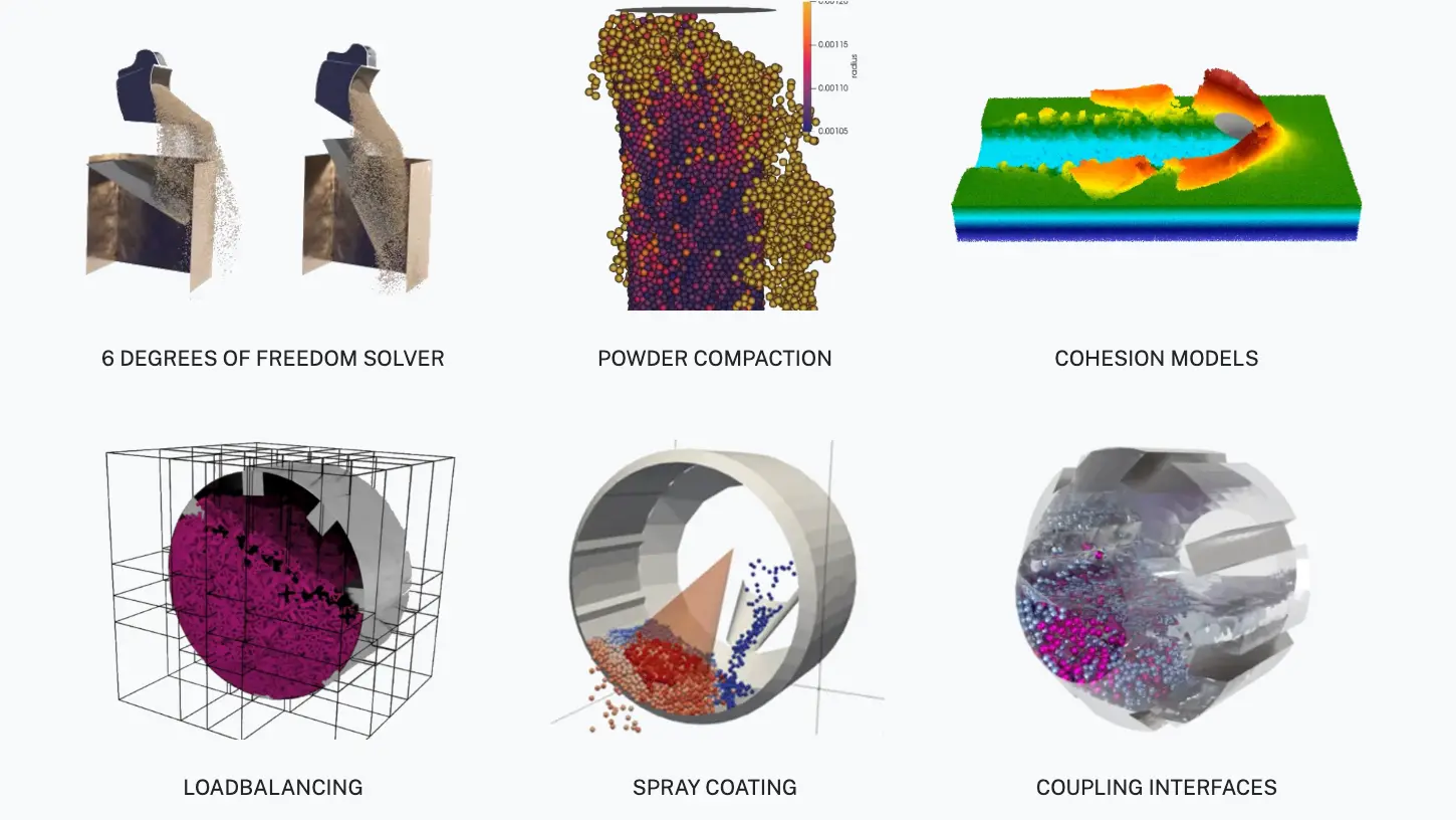
Explore our Features
Discover powerful tools and technologies designed to enhance your simulations.
References
Hear from satisfied customers about the impact our solutions had on their success.
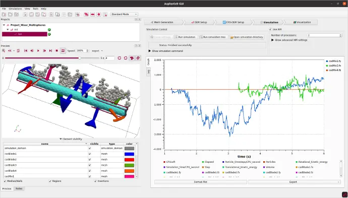
Consultancy
We’ll provide expert answers and introduce our software, always pushing simulation boundaries.